A Review of Introduction to Kolmogorov-Arnold Network(KAN)

Abstract

In the past 60 years Multi-Layer Perceptron(MLP) has helped us as the fundamental block of deep learning based on the approximation theorem. Though MLP suffered from a critical lacking of interpretability and require massive parameter often. This article explores Kolmogorov-Arnold Network(KAN) model which was proposed in 2024. This Model was proposed by Andrey Kolmogorov and Vladimir Arnold. Previously MLP placed Fixed Activation functions on nodes but KAN Place Learnable Activation functions on edges. Here we will analyse the mathematical difference between these two architectures by examining the use B-Splines on edge and weights and we will also discuss How KAN offered us promised path towards the "White Box" AI that is very much accurate and interpretable.

Introduction

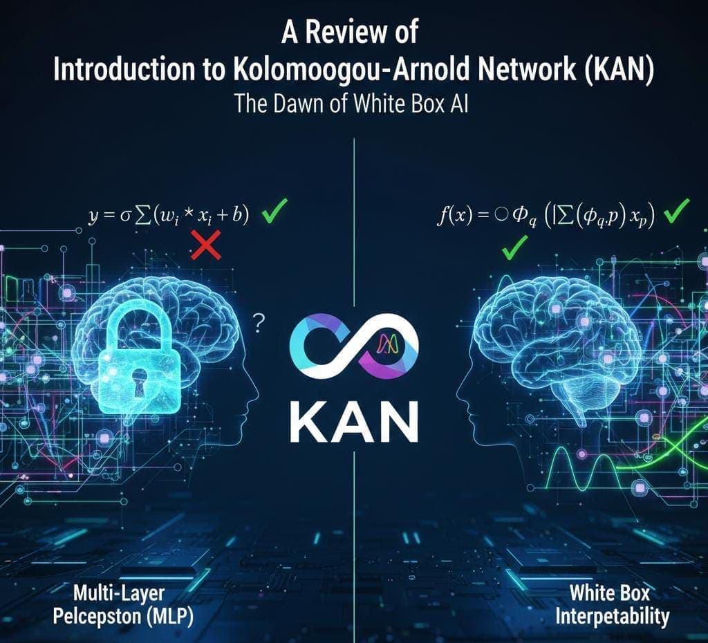
1. Stagnation of Perceptron These neural network is built on a mathematical assumption specifically that is the linear combination of Inputs Based on Fixed nonlinearity. In standard MLP, we define a neural computation as: $y = \sigma \left( \sum_{i=1}^n w_i x_i + b \right)$ Here:

• $w_i$ Indicates Learnable Scalar weights.
• $\sigma$ Indicates Fixed activation function.

These structure Took help From the activation function by making it a static Gatekeeper. This structure results In Black box while universally approximating where Specific contribution of features is calculated by layers of matrix multiplication.

2. Mathematical Foundation To understand KAN We focused 2 fundamental mathematical theorem.

• Universal Approximation Theorem (MLP Basis): MLP Calculates that Sum of all nonlinear function can give an approximate result to any continuous functions.
• Kolmogorov-Arnold Theorem (KAN Basis): KAN states that any multivariate continuous function lie on a bounded domain can be represented as a finite composition of multiple univariate functions. $f(\mathbf{x}) = f(x_1, \dots, x_n) = \sum_{q=0}^{2n} \Phi_q \left( \sum_{p=1}^n \phi_{q,p}(x_p) \right)$ In this formula:
• $\phi_{q,p}$ are univariate functions (functions of a single variable).
• $\Phi_q$ is the aggregation function.

Architecture

The first innovation on KAN is by replacing the linear weight with a learnable non-linear function.

• The Activation Age: In MLP if an
  age = X
  and
  Skills Scales = W
  . Then in KAN an
  age = X
  and transforms it via a function $\phi(x)$.
• Basic Splines(B-Splines) Implementation: We cannot learn from an arbitrary function directly from code, so we will approximate these functions by using B-Splines, which are piecewise polynomial functions defined by control points. The learnable function $\phi(x)$ is expressed as: $\phi(x) = \sum_i c_i B_i(x)$ Where:
• $B_i(x)$ are the fixed basis functions (the spline shape).
• $c_i$ are the learnable coefficients (control points).

Pseudocode

# 2. The KAN Approach (Learnable Edges, Summing Nodes)
class KAN_Layer:
    def forward(self, x):
        # Step A: Apply Learnable Non-Linear Functions
        # Instead of multiplying by a scalar 'W', we apply a function 'phi'
        # 'phi' is built using B-Splines (basis functions)
        
        # logic: y = sum(phi(x))
        
        # We compute the shape of the function based on learnable coefficients
        spline_basis = compute_b_splines(x)
        phi_x = spline_basis * self.spline_coefficients
        
        # Step B: Summation
        # The node simply sums up the incoming function results
        y = sum(phi_x)
        return y

Advantages

1. White box interpretability: We know that every edge is a univariate function that we can see exactly how one input variable affects the other output variable. In MLP Feature interactions are ignored in weight matrices, but KAN allows us to plot one spline shape on every connection. For example, if spline shapes look like a parabola we confirm it is a quadratic relationship; if it shapes like a sinusoidal then we confirm the relationship is periodic.
2. Parameter efficiency: In Symbolic Regression KAN helps by reaching lower loss values with fewer parameters than MLPs. A small KAN often discovers a physics law where a large MLP only poorly approximates the curve without understanding its structure.

Conclusion

KAN shows a paradigm shift from learning linear weights to learning functions by using the Kolmogorov-Arnold Theorem and B-Splines. KAN offers us a glimpse into the future of interpretable Artificial Intelligence. Though currently training slower than MLPs due to the complexity of calculating splines, they provide a bridge over the gap between deep learning and symbolic mathematics. For an AI engineer studying KAN will help rethink the atomic unit of neural computation.